On Invariance and Inconsistency

Section 1. Introduction

How can you explain important concepts from program correctness in a simple and intuitive manner? In this blog post, we shall have a look at some puzzles and analyze them from the perspective of program correctness. This way we can nicely explain and demonstrate the usefulness of two important concepts, namely invariants and (in)consistent specifications.

The puzzles we study here come from the book Algorithmic Puzzles by Anany and Maria Levitin, published by Oxford University Press in 2011. This book presents 150 puzzles that are good candidates for applying analytical and logical thinking skills (the puzzles can also be used as challenging interview questions). We make a small selection of the puzzles, and we will see them answered from the perspective of program correctness. In program correctness, we consider a program to be correct with respect to a given program specification. A program specification is a specific formulation of a requirement. For example, a specification of what the output of a program must be given some input. More specifically (no pun intended), we can rephrase the puzzles in such way that a puzzle can seen as a program specification, and proving that there exists a program that is correct with respect to that specification would then solve the puzzle in question. Or, alternatively, we show that there is no solution to the puzzle, by arguing there cannot be a correct program in the first place.

First we shortly revisit preliminaries (Section 2). This article does assume the reader is already somewhat familiar with the basics of programming and program correctness, but we nevertheless quickly revisit the basic concepts. For a thorough introduction to program correctness, one could take a look at one of the following books (in order of appearance):

• A Discipline of Programming by Edsger Dijkstra (1976),
• Mathematical Theory of Program Correctness by Jaco de Bakker (1980),
• The Science of Programming by David Gries (1981),
• Program Verification by Nissim Francez (1992), or
• Verification of Sequential and Concurrent Programs by Krzysztof Apt, Frank de Boer & Ernst-Rüdiger Olderog (2009).

Then we shed light on the concept of an invariant by discussing the 5th puzzle of the book, ‘Row and Column Exchanges’ (Section 3). We also look at why declarative specifications are useful by discussing the 12th puzzle of the book, ‘Questionable Tiling’ (Section 4). But we also discuss more generally the importance of invariants and formulating consistent specifications (Section 5).\(\def\Coloneqq{\mathrel{::=}}\def\coloneqq{\mathop{:=}}\def\llbracket{{[\![}}\def\rrbracket{{]\!]}}\)

Section 2. Preliminaries

We shall restrict our attention to a simple imperative programming language: \[\begin{gathered} S \Coloneqq x \coloneqq a \mid S_1;S_2 \mid \mathbf{if}\ b\ \mathbf{then}\ S_1\ \mathbf{else}\ S_2\ \mathbf{fi} \mid \mathbf{while}\ b\ \mathbf{do}\ S\ \mathbf{od}\end{gathered}\] where we use not only \(x\) as variable but also \(y,z,\ldots\) (possibly with subscripts), where the terms \(a\) of the language are the usual arithmetical expressions: \[\begin{gathered} a \Coloneqq 0 \mid 1 \mid x \mid -a \mid (a_1 + a_2) \mid (a_1 \times a_2)\end{gathered}\] and where the terms \(b\) of the language are the Boolean expressions: \[\begin{gathered} b \Coloneqq (a_1 = a_2) \mid (a_1 < a_2) \mid (b_1 \land b_2) \mid (b_1 \lor b_2) \mid \lnot b\end{gathered}\] We also have the usual abbreviations, such as \((a_1 \leq a_2)\), that abbreviate more complex expressions, such as \((a_1 < a_2) \lor (a_1 = a_2)\), respectively. The numerals \(2,3,4,\ldots\) are also abbreviations of complex expressions \((1+1), (1+2), (1+3),\ldots\)

We also have first-order formulas, captured by the following syntax: \[\begin{gathered} \phi,\psi \Coloneqq b \mid (\phi \to \psi) \mid (\forall x)\phi\end{gathered}\] Other logical connectives, such as \((\phi \land \psi)\) and \(\lnot\phi\), can seen as abbreviations. First-order logic involves first-order universal quantification \((\forall x)\phi\), and we have the dual of first-order existential quantification \((\exists x)\phi\) as abbreviation of \(\lnot(\forall x)\lnot\phi\). Quantification only ranges over individuals, so in our case integers.

Now let us consider semantics. Let \(\sigma\) be a state (an assignment of variables to integer values). We have the usual semantics for arithmetical expressions \(a\) and Boolean expressions \(b\): \(\llbracket a \rrbracket_\sigma\) denotes an integer value and \(\llbracket b\rrbracket_\sigma\) denotes a Boolean value. Note that an expression depends only on finitely many variables, and we only deal with pure expressions in our simple language. Each statement \(S\) of our programming language denotes a transition relation of states: \[\llbracket S\rrbracket \subseteq \Sigma\times\Sigma\] where \(\Sigma\) is the set of states (with typical element \(\sigma\)), and \(\Sigma\times\Sigma\) is the set of pairs of states. A statement denotes a binary relation between initial and final states. Each formula \(\phi\) denotes a set of states: \[\llbracket \phi\rrbracket \subseteq \Sigma\] in the sense that in each state \(\sigma\in\llbracket\phi\rrbracket\) the formula \(\phi\) is true, also written \(\sigma\models\phi\).

In program correctness we combine two languages: a programming language and a specification language. The programming language is already given above. As specification language we take the above first-order language. Note that the variables of formulas in the assertion language are the same variables we use in the programming language. We can now form the Hoare triples: \[\{\phi\}\ S\ \{\psi\}\] where \(\phi\) is called the precondition and \(\psi\) is called the postcondition. A Hoare triple is correct when the statement \(S\) satisfies the input/output specification given by the precondition \(\phi\) and the postcondition \(\psi\), and a Hoare triple is incorrect otherwise. Note that the (global) variables of \(S\) and the (free) variables of the formulas \(\phi\) and \(\psi\) are bound to each other. Formally, we define \[\models \{\phi\}\ S\ \{\psi\} \text{ if and only if } \llbracket S\rrbracket(\llbracket\phi\rrbracket) \subseteq \llbracket\psi\rrbracket\] where \(R(X)\) is the left-restriction of the binary relation \(R\) by the set \(X\), that is, \(R(X) = \{y \mid xRy\text{ for some }x\in X\}\). Unpacking this formal definition gives us \[\models \{\phi\}\ S\ \{\psi\} \text{ if and only if } \sigma\in\llbracket\phi\rrbracket \text{ and } (\sigma,\tau)\in\llbracket S\rrbracket \text{ implies } \tau\in\llbracket\psi\rrbracket.\]

Incorrectness means that \(S\) has a bug. Suppose we start in some initial state \(\sigma\) which satisfies the precondition \(\phi\), and we execute \(S\) from that state, and that execution results in some final state \(\tau\). If the final state \(\tau\) does not satisfy \(\psi\), then we have found a bug! Formally, \[\not\models \{\phi\}\ S\ \{\psi\} \text{ if and only if } \sigma\models\phi \text{ and }(\sigma,\tau)\in\llbracket S\rrbracket\text{ and }\tau\not\models\psi\text{ for some }\sigma,\tau.\]

Hoare logic is a formal system in which Hoare triples can be derived, in which case one writes \(\vdash \{\phi\}\ S\ \{\psi\}\). Hoare logic is sound and (relatively) complete, meaning that we have \[\vdash \{\phi\}\ S\ \{\psi\}\text{ if and only if }\models \{\phi\}\ S\ \{\psi\}\] under some reasonable assumptions.¹ See one of the books mentioned in in the introduction for a presentation of Hoare logic, or Wikipedia.

A quick example is the following Hoare triple. Is it correct or not? \[\{y = 0\}\ x \coloneqq 1; \mathbf{while}\ x \leq z\ \mathbf{do}\ y \coloneqq y + x; x \coloneqq x + 1\ \mathbf{od}\ \{2\times y = z\times(z+1)\}\] To verify the loop, we need to come up with a so-called loop invariant: a condition that holds at four control points (1) before entering the loop, (2) before the loop body begins, (3) after the loop body ends, and (4) after the loop is exited. Finding loop invariants is difficult, and often it takes multiple tries until one finds a suitable invariant. In the above example, one can take: \[1 \leq x \leq z + 1 \land 2\times y = (x - 1)\times x\] where \((x - 1)\) abbreviates \((x + -1)\) and the chain of inequalities is conjunctive.

Section 3. Invariants

In this section we discuss a puzzle in which invariants play a prominent role. The 5th puzzle of the book Algorithmic Puzzles is ‘Row and Column Exchanges’:

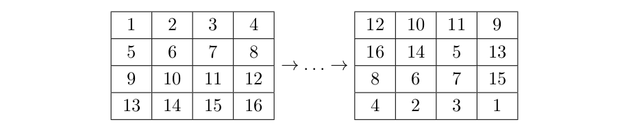
Can you transform the left table into the right table of Figure 1 by exchanging its rows and columns?

(It is recommended that the reader first tries out solving this puzzle herself!)

To get a sense of what the puzzle asks for, let us perform the operations of swapping rows and columns in a table. An example of a sequence of successive applications of these operations is shown in Figure 2.

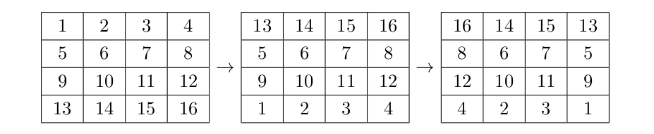
This figure shows:

1. The first table shows the initial table of Figure 1, our starting point in this puzzle.
2. After the first step, we have exchanged the first and last row. So we swapped the values \(1,2,3,4\) and \(13,14,15,16\).
3. After the second step, we have also exchanged the first and last column. So we swapped the values \(13,5,9,1\) and \(16,8,12,4\).

Notice that we have now obtained a table, in which the last row coincides with the values of the final table we wish to obtain (the last row is ‘correct’ with respect to the desired final table). To get closer to the final table, we can continue the series of operations as in Figure 3, where we perform two additional steps: we swap the first and third row, and we swap the second and third row.

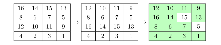
In the resulting table, we have colored the cells that have values in the right place when comparing it to the final table in Figure 1. This particular example shows that we are not there yet. Click here for a Rust implementation of this example.

Just giving this single example, where we have not solved the puzzle (since the final table is not ‘correct’), is not a solution the puzzle! But one may wonder, whether there exists a solution at all. If there exists a solution, then we have not yet found it. But, if there is no solution to be found, then just showing this single counter-example is not sufficient proof.

Imagine that these tables are representations of state, where the state is an assignment of integers to variables (each cell in the table is modeled by its own variable, sixteen in total). There are two primitive operations that work on this state:

• to swap two columns \(C(j,j')\), and
• to swap two rows \(R(i,i')\).

The puzzle can be rephrased by asking whether we can come up with a program that is composed out of these two primitive operations. Instead of our simple programming language given above, where the only primitive operation is the assignment \(x := a\), we instead consider the programming language with only these two primitive operations. In this way we realize encapsulation, in the sense that the program may not directly modify the state by means of an assignment, only indirectly through the exposed operations.

This may remind the reader of object-oriented programming. Each table could be seen as an instance of a class of objects, which has an encapsulated internal state. The class of objects exposes a number of operations, viz. it has a well-defined interface. We ask ourselves now: does there exist a client, which can only work with the interface and not directly modify the internal state, that solves our puzzle?

What does it mean to solve the puzzle? We can formulate the Hoare triple \[\{\!\!\!\bigwedge_{i\in[1,4]}\bigwedge_{j\in[1,4]}\!\!\!x_{i,j} = (i - 1) \times 4 + j\}\ S\ \{x_{1,1} = 12 \land \ldots \land x_{4,4} = 1\}\] where \(x_{1,1}\) until \(x_{4,4}\) are the sixteen variables corresponding to the cells of the table.² Note that in the postcondition we simply require the variables to have the proper values, as indicated in Figure 1. If we can find a program \(S\) that is composed of only these primitive operations, and prove it correct, we have solved the puzzle!

To understand the meaning of the primitive operations, we give a set of Hoare triples that we take as axioms (technically, we give an axiom scheme). This approach is also known as the ‘axiomatic approach’, where we abstract from the exact semantics of the primitive operations. Here we go (assuming meta-variables \(j\in[1,4]\) and \(j'\in[1,4]\)): \[\{\!\!\!\bigwedge_{i\in[1,4]}\!\!\!x_{i,j} = y_r \land \!\!\!\bigwedge_{i\in[1,4]}\!\!\!x_{i,j'} = z_r\}\ C(j,j')\ \{\!\!\!\bigwedge_{i\in[1,4]}\!\!\!x_{i,j} = z_r \land \!\!\!\bigwedge_{i\in[1,4]}\!\!\!x_{i,j'} = y_r\}\] The ‘freeze variables’ \(y_1,\ldots,y_4\) capture the old values at column \(j\), and \(z_1,\ldots,z_4\) capture old values at column \(j'\). In the postcondition, we use the (unchanged) freeze variables to refer to the old values at the beginning of the swapping operation. This argument crucially relies on the fact that the operation \(C(j,j')\) only changes the variables in the set \(\{x_{i,j},x_{i,j'}\mid i\in[1,4]\}\). By Hoare’s invariance rule, we know that any property about the other variables thus remains invariant. A similar axiom scheme can be given for swapping the rows.

We could think of an object invariant: a property that holds of the internal state of the object, that must be preserved by every operation that is performed by any client. Note that object invariants may be temporarily broken in the implementation of an operation, as long as the object invariant is restored before the implementation terminates.

The beauty of invariants is that they are a powerful tool for answering these kinds of puzzle questions. When we are able to find some invariant, that is true for the initial table but false for the final table, then we must know: the final table cannot be obtained by means of these operations only, since all the operations preserve the object invariant!

An example of an object invariant in this case would be the property: the table has the values \(\{1,\ldots,16\}\). In other words, every value in the table is in \(\{1,\ldots,16\}\) and every value of \(\{1,\ldots,16\}\) is somewhere in the table. Let’s formalize it: (Eq.1) \[\{x_{i,j} \mid 1\leq i,j \leq 4\} = \{1,\ldots,16\}.\label{eq:obj-inv}\] The set comprehension on the left collects all values in the table in a set. The set expression on the right is the finite set consisting of the integers \(1\) up to and including \(16\). The property now expresses that these two sets are identical, i.e. have precisely the same members. This property holds for the initial state of the object, and it also is preserved by every operation: swapping two rows, or swapping two columns, does not introduce any new values and thus does not invalidate this property. Hence, this property is an object invariant.

The final table of Figure 1 also satisfies the object invariant in the equation (Eq.1) above. So this invariant, while nice to know, is not useful in answering the puzzle question. We can only prove that there is no solution to the puzzle when we find an invariant, that holds of the initial state and is preserved by the operations, but does not hold in the final state.

Just how finding loop invariants (to show the correctness of a program) is a difficult problem, finding object invariants (to show there can be no correct program) is also a difficult problem. Finding invariants may require several tries. Let us try another invariant. Consider that we not only have a set of values, but in fact we have a set of sets of values: \[\bigl\{\{x_{i,j} \mid 1\leq i\leq 4\}\mid j \leq 4\bigr\} = \bigl\{\{1,2,3,4\},\ldots,\{13,14,15,16\}\bigr\}\] The outer set consists of the sets corresponding to the values one finds at each row. And the inner sets consists of the values present at each row. If we swap two rows, the invariant is preserved because the outer set does not care about the order of its values (sets of integers). If we swap two columns, then the invariant is preserved, because the set of values at each row remain the same when we have swapped two columns.

Now, looking at Figure 1 we see that the initial table satisfies this property. However, if we look at the final table we see that it does not satisfy this property. The final table has as set of sets of integers: \[\bigl\{\{12,10,11,9\},\{16,14,15,13\},\{8,6,7,5\},\{4,3,2,1\}\bigr\}.\] Sure, the first and last row are correct, so we could focus on comparing the sets \[\bigl\{\{16,14,5,13\},\{8,6,7,15\}\bigr\} \text{ and } \bigl\{\{16,14,15,13\},\{8,6,7,5\}\bigr\}\] which cannot be equal because both sets contain values that are not contained in the other set. Hence the final table does not satisfy the invariant, which finally proves that there is no solution! (We shall further discuss this problem in Section 5.)

Section 4. Logical Specifications

We have a look at the 12th puzzle of the Algorithmic Puzzles book, ‘Questionable Tiling’ (with a slightly different phrasing):

Is it possible to tile an 8-by-8 board with dominoes (2-by-1 tiles) such that no two dominoes lie next to each other in parallel?

(Again, the reader should first try to solve this puzzle herself!)

Before even beginning to solve the problem, we should first try to get an exact understanding of the puzzle by understanding each part of the question:

• What is a ‘tiling of dominoes’ on an 8-by-8 board?
• What does it mean when two dominoes ‘lie next to each other in parallel’?

Suppose we formalize the 8-by-8 board, again by means of a table. Each cell of the table is again understood to be represented by the variables \(x_{i,j}\) where \(i\) is the row counted from the top and \(j\) is the column counted from the left. But what do the values of these variables mean? We could devise the following encoding:

• If a variable \(x_{i,j}\) has value \(0\) it means that the cell is empty.
• If a variable \(x_{i,j}\) has some positive value, then that positive value identifies a domino piece.

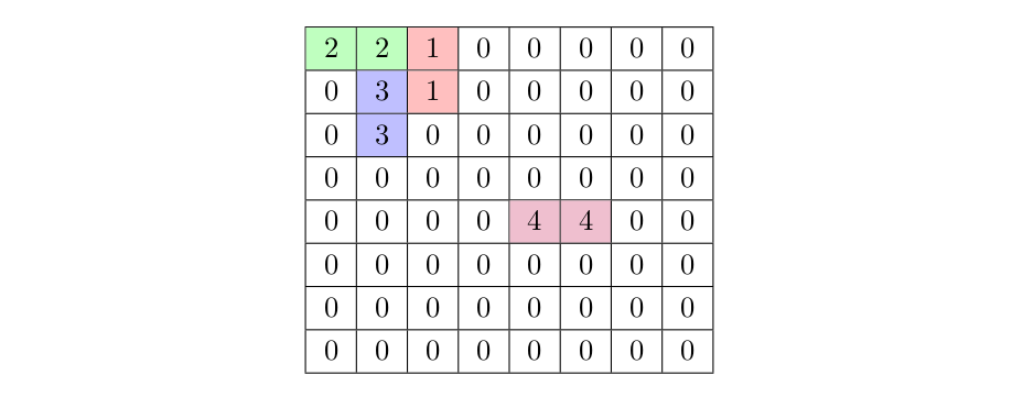
For example, see Figure 4 where we have a table that encodes an 8-by-8 board with only four dominoes. Note that in this and the following pictures, only the numbers in the cells are significant and not the colors. Colors are only for visual aid. Further, what is shown in Figure 4 is not a tiling yet, it is a partial tiling and towards becoming a complete tiling.

One fruitful approach would be looking for patterns. A pattern is, figuratively speaking, a small ‘frame’ or ‘scope’ that you locally could observe in the picture. These patterns are ‘timeless’ and observed of the outcome, and thus do not care about the intermediary state one has passed through to obtain the outcome. Finding patterns is a useful ability of a declarative programmer.

One can observe already the following properties:

Property 1. (Number of dominoes in tiling)
In an 8-by-8 table, a complete tiling has exactly \(\frac{8\times 8}{2}=32\) numbers identifying domino pieces.

Property 2. (Size of single domino)
Every number identifying a domino piece occurs at most twice.

Property 3. (Dominoes line up)
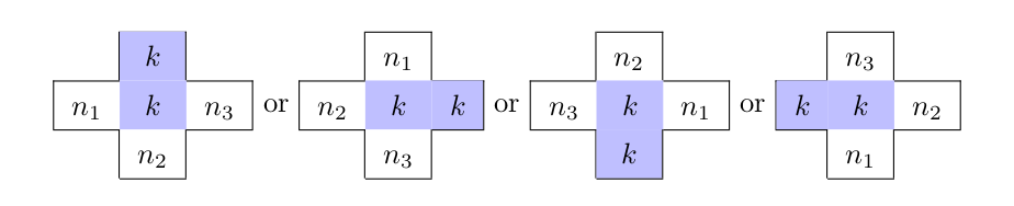
Given a cell of a table that contains a number identifying a domino. Now consider its immediate neighborhood (the cells on the top, right, bottom, left—but not the diagonal cells). We observe that the following must hold: a cell above, on the left, below, or on the right of the given cell exists and has the same domino identifying number. The other neighboring cells must have a different value. See also Figure 5 for a picture, but note that these patterns only work for interior cells. For cells on the border, the pattern need not check outside bounds.

Now, consider completing the tiling in Figure 4. What domino do we place on the left of the domino identified by number three (the blue one)? It will form a 2-by-2 square. We also form a 2-by-2 square if we would place another domino directly below and in parallel with the domino identified by number four (the purple one). These are undesired according to the puzzle.

We end up with the following property:

Property 4. (No parallel dominoes)
In each 2-by-2 square there are not exactly two dominoes. See Figure 6 for the two forbidden patterns.

We can now formalize the properties, and obtain a program specification.

Property 1. (Number of dominoes in tiling) \[|D| = 8\times 8\] where \(D\) is the set of domino identifying numbers that occur somewhere in the table, that is, \(D = \{x_{i,j} \mid 1 \leq i,j\leq 8\}\cap\{n\mid n > 0\}\).

Property 2. (Size of single domino) \[|\{(i,j) \mid k = x_{i,j}\text{ and }1\leq i,j\leq 8\}| = 2\text{ for each }k\in D.\]

Property 3. (Dominoes line up)
For every \(1\leq i,j\leq 8\) there is some \(\ell\in K(i,j)\) such that \[x_{i,j} = x_\ell \land\mkern-28mu\bigwedge_{k\in K(i,j)\setminus\{\ell\}}\mkern-20mu x_{i,j}\neq x_{k}\] where \(K(i,j)\) is the set of neighboring coordinates within bounds \[\{(i+1,j),(i,j+1),(i-1,j),(i,j-1)\} \cap \{(i',j')\mid 1\leq i',j'\leq 8\}.\]

Technically, we have that \(x_{(i,j)}\) is defined to be equal to \(x_{i,j}\) so we can use the coordinates to refer to a particular subscripted variable.

Property 4. (No parallel dominoes)
For every \(1 \leq i,j < 8\) we have \[|\{x_{(i,j)},x_{(i+1,j)},x_{(i,j+1)},x_{(i+1,j+1)}\}\cap\{n\mid n > 0\}| \neq 2.\]

These properties can be abbreviated to \(P1,P2,P3,P4\), respectively. Now the puzzle amounts to finding a program \(S\) that changes the variables \(x_{1,1},\ldots,x_{8,8}\) such that we can prove \[\{\mathbf{true}\}\ S\ \{P1\land P2\land P3\land P4\}.\] Consider a program that assigns the cells’ values according to Figure 7. We can now verify whether the program indeed satisfies the specification, by checking whether all properties hold.

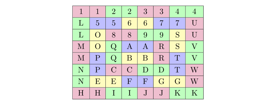
\(P1\) holds because there are exactly 32 dominoes in the final state assigned to the variables. \(P2\) holds since every number identifying a domino piece occurs exactly twice. Also \(P3\) holds, and this can easily be seen by the different colors. However, checking \(P4\) shows that the property is violated (see the center).

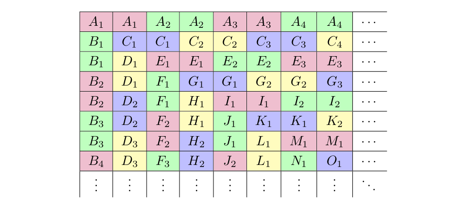
If we slightly generalize the problem, then we see there is a solution. Suppose the board is infinite, i.e. we have an \(\infty\)-by-\(\infty\) board, which we start tiling from the top-left corner. Then the following brick laying pattern can be continued indefinitely (see Figure 8):

• Start horizontally with the dominoes \(A_1,A_2,\ldots\) and lay the next on the right of the previous one until the entire first row is covered with dominoes.
• Continue vertically with the dominoes \(B_1,B_2,\ldots\) and lay the next below the previous one until the entire first column is also covered with dominoes.
• We are now in the same situation as before: we want to fill an \(\infty\)-by-\(\infty\) board, so we repeat the strategy of first laying \(C_1,C_2,\ldots\) horizontally and then laying \(D_1,D_2,\ldots\) vertically.

Such an infinite board would then satisfy these properties:

• The number of dominoes on the infinite board are also infinite.
• If we make sure that each domino is represented by a different number, then each such number occurs only twice. For example, we could take the numbering scheme where for each domino that lies on the coordinates \((i,j)\) and \((i',j')\) we take as identifier \(\min(2^i3^j,2^{i'}3^{j'})\).
• The dominoes are placed correctly, as can be observed from the coloring.
• There are no parallel dominoes, since each 2-by-2 square has exactly three dominoes.

Note that we avoided the occurrence of four dominoes within a 2-by-2 square, as shown in Figure 9.

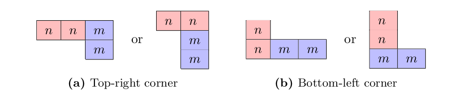
More generally, we never have any of the patterns in Figure 10 occurring. These patterns are called the top-right corner and bottom-left corner. Note that these patterns do occur in Figure 9, so already from knowing the absence of these two corners we also know that there can be no four different dominoes within a 2-by-2 square.

Now suppose we would cut off the board of Figure 8 so to obtain an 8-by-8 board. We then see problems occurring at the boundaries, with dominoes sticking out. Here are two instances:

1. On the first column, we see that the domino \(B_4\) falls out of bounds. Hence the only way to lay down that domino is by turning it 90 degrees.
2. On the second row, we see that the domino \(C_4\) also falls out of bounds. Also here we would need to lay down that domino turned by 90 degrees.

What we thus see, is that whenever the board is finite, it must have one of the corners of Figure 10. We shall now argue that it is impossible to satisfy \(P4\), the property that no dominoes are parallel, whenever we have the (necessary) top-left corner and also either the bottom-left or the top-right corner on the board. We make a number of simplifying assumptions, but these do not hurt our demonstration (that is to say, these assumptions are without loss of generality):

• we assume we work on an arbitrary \(n\)-by-\(n\) board where \(n\) is even,
• we assume we start with the same type of top-left corner and top-right corner where the horizontal domino is on top,
• we assume that both corners occur on the same height.

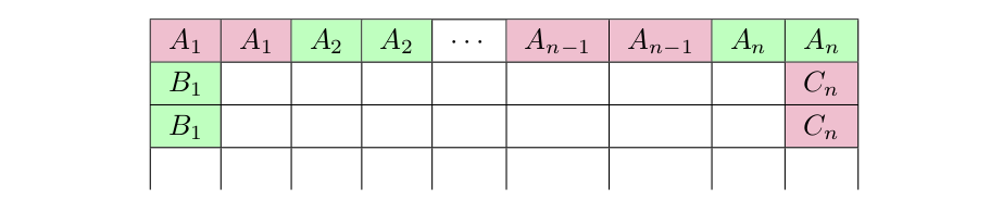
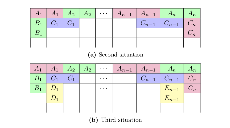
Now consider the situation of Figure 11. Consider that, if we were to satisfy all properties \(P1\) until \(P4\), it is impossible to place a domino vertically next to \(B_1\) nor is it possible to place a domino vertically next to \(C_n\). If we were to place a domino horizontally at the low end at \(B_1\) (thus forming a bottom-left corner), then we need to place another domino on top that violates \(P4\). Hence the only dominoes that are possible are depicted in Figure 12a. We end up with the other type of corner (where the vertical domino is on the side) and we can again analyze where to place the next domino in the corner next to \(B_1\) and below \(C_1\), and next to \(C_n\) and below \(C_{n-1}\). After analyzing the possibilities and ruling out those that violate \(P4\) we end up with the situation depicted in Figure 12b.

After continuing this way, we see that we construct two ‘lines’, one originating from each corner. It is necessarily the case that these two lines will intersect!

In Figure 13 we see the two lines coming diagonally out of the top-left corner and the top-right corner intersect. The way this plays out is as follows: we start with the corner consisting of dominoes \(\{1,2\}\) (the top-left corner) and dominoes \(\{A,B\}\) (the top-right corner). Then we necessarily place domino \(3\), but this takes the same place as we would take when we would place a domino in the other corner. We now have two corners, but they share a domino, namely the dominoes \(\{2,3\}\) (the top-left corner) and the dominoes \(\{3,B\}\) (the top-right corner). We then place \(4\) and \(D\) in the only way possible inside these corners, but we see that this gives us a parallel pair of dominoes in a 2-by-2 square.

Summarizing, the argument goes as follows. If there are two corners on the board that induce a ‘diagonal line’ that intersect, this must give rise to a pair of parallel dominoes. Hence we can not have both a top-left corner and a top-right corner on the board. However, for every \(n\)-by-\(n\) board tiling it is necessary to have both a top-left corner and a top-right corner. Hence we cannot have a tiling of the 8-by-8 that also has no parallel dominoes.

Section 5. Conclusion

We have now seen two example puzzles, which we phrased by means of asking whether we can come up with a program that satisfies certain requirements. In the first example (Section 3) we have seen that the program’s requirements can (1) be stated formally, and (2) a final state was imaginable that satisfies the end goal, but (3) there was no correct program that reaches the final state. In the second example (Section 4) we have seen that the requirements themselves can (1) be stated formally, but already that (2) a final state was not imaginable that satisfies the end goal. If there is no final state that satisfies the requirements, it is impossible to write a correct program. This must be a valid conclusion, since each program only moves from state to state, and there does not even exist a state that satisfied the requirements.

All this serves to show is that program correctness is a difficult subject. It shows that sometimes it is ‘easy to ask’ but ‘difficult to deliver’. Extensive analysis of a problem is required to obtain (1) a formal description of the problem, and (2) proof that the requirements are consistent. Even before one starts writing a program, one already has to face an undecidable problem: namely, to check that the requirements are consistent! And we have seen a concrete example that this is not always the case—even when the problem looks simple. If we then have requirements that are satisfiable, we then face the second difficult problem: does there exist a correct program? We have seen that, no, this is not obvious either. To show that there does not exist a correct program, we need to formulate an invariant that any program preserves but which the final state violates. On the other hand, whenever there exists a non-trivial program (i.e. involving a loop) we also face a difficult problem: to prove it correct requires us to come up with an invariant as well.

This finally gives us two slogans:

To show a program is correct, requires one to find an invariant. To show there is no correct program, also requires one to find an invariant.

and

Correctness is impossible to attain if the requirements are inconsistent.

Bonus questions.

1. Can you analyze the problem of swapping rows and columns also in the context of concurrent client programs?
2. What about tiling the board without parallel dominoes when the boundaries are glued to each other in weird (non-Euclidean) ways?

1. Access to an oracle that provides the valid formulas in arithmetic (this is an undecidable problem), and the expressivity of loop invariants.↩︎

2. Technically, the ‘quantifiers’ in the precondition are not first-order quantifiers but instead abbreviations where \(i\) and \(j\) are meta-variables that range over finitely many constant values: thus the formula is a big conjunction with sixteen clauses where each clause specifies the value of precisely one variable.↩︎