Correctness of Two Sorting Algorithms
This article describes two sorting algorithms (gnome sort and bozosort) and gives their correctness proof in full detail.
On Wednesday, 8th of March, 2023, I gave a lecture about two sorting algorithms for the course Program Correctness (see also the lecture series on YouTube, available only in Dutch). Then, due to limited time, I only discussed a sketch of the correctness proof. But I promised the students that I would write down the correctness argument in more detail. So, in this article, I will revisit the two sorting algorithms and give the correctness proof in full detail.
We had a look at two sorting algorithms: gnome sort and bozosort. The purpose of a sorting algorithm is to operate on an array and rearrange its elements in order. The two algorithms presented are not the most efficient sorting algorithms, but that is not of our concern: instead, we will look at them from the perspective of their correctness.
The main questions answered in this article are:
- What is the (intuitive) argument of correctness of these algorithms?
- How to write down a proof outline for these algorithms?
When proving an algorithm correct, it is important to first have a rough, informal, idea how the correctness argument should go. Only then it makes sense to formalize the argument, by writing down a proof outline. During the latter activity, one can systematically check the argument to ensure there is no fault in one's own reasoning. Thus, both aspects are important: the bigger picture and the devil's in the details.
Sorting
The purpose of a sorting algorithm is to rearrange elements in an array, so that the final result is an array where all elements are in order. For simplicity, we assume we are dealing with an array of integers. The ordering of integers is their natural order, i.e. \(\ldots\leq -2\leq -1\leq 0\leq 1\leq 2\leq \ldots\).
Given array \(a\) of type \(\mathbf{integer}\to\mathbf{integer}\). We define the following predicate: \[\mathit{Sorted}(a) \equiv_\mathrm{def} \forall i, j : i \leq j \to a[i] \leq a[j].\] The above predicate expresses that the whole array \(a\) is sorted. We also define: \[\mathit{Sorted}(a,f,t) \equiv_\mathrm{def} \forall i, j : f \leq i \leq j \leq t \to a[i] \leq a[j].\] This predicate expresses that array \(a\) is sorted on the range \([f,t]\), i.e. from index \(f\) until and including index \(t\).
Alternatively, we can define the following predicates: \[\mathit{Sorted}\,'(a) \equiv_\mathrm{def} \forall i : a[i] \leq a[i + 1]\] and \[\mathit{Sorted}\,'(a,f,t) \equiv_\mathrm{def} \forall i : f \leq i < t \to a[i] \leq a[i + 1].\] It can now be verified (e.g. using a proof system for predicate logic such as natural deduction) that \(\mathit{Sorted}(a) \equiv \mathit{Sorted}\,'(a)\) and \(\mathit{Sorted}(a,f,t)\equiv\mathit{Sorted}\,'(a,f,t)\).
We may use these predicates to describe the desired outcome of a sorting algorithm: namely, that array \(a\) is sorted (on a particular range). However, this property alone is not sufficient. We also require a relation between the input array and the output array, to specify that the algorithm did not insert new, duplicate old, or throw out any elements. Note that the input array and the output array are stored in the same place in memory, so it matters not where we look but when we look. By input array we mean the value of the array \(a\) before the algorithm runs, and by output array we mean the value of the (same) array \(a\) but after the algorithm finished running.
To avoid algorithms inserting new, duplicating old, or throwing out elements, we require there exists a one-to-one correspondence between the input and output array.
Given array \(b\) of type \(\mathbf{integer}\to\mathbf{integer}\). We use \(b\) as the name for the input array, whereas \(a\) is the name for the output array. We now define the following predicate: \[\mathit{Permut}(a,b) \equiv_\mathrm{def} \exists \pi : \mathit{Inj}(\pi) \land \mathit{Surj}(\pi) \land \forall i : b[\pi(i)] = a[i].\] This predicate expresses that the whole array \(a\) is a permutation of array \(b\). The intuition of \(\mathit{Permut}(a,b)\) is that \(\pi\) represents a bijection between integers: a one-to-one correspondence between the indices of the output array \(a\) and input array \(b\). Here we make use of the following definitions: \[\mathit{Inj}(\pi) \equiv_\mathrm{def} \forall x, y : \pi(x) = \pi(y) \to x = y\] and \[\mathit{Surj}(\pi) \equiv_\mathrm{def} \forall x : \exists y : \pi(y) = x.\]
(As an aside, i.e. not relevant for the rest of this article, note that it depends on the language in which we work whether quantification over \(\pi\) is first-order or not. If we work in the language of Peano arithmetic, this quantifier is higher-order. But if we work in the language of set theory, this quantifier is first-order where \(\pi\) ranges over sets representing functions \(\mathbf{integer}\to\mathbf{integer}\).)
We actually need a stronger predicate than \(\mathit{Permut}\), namely to expresses that array \(a\) is a permutation of array \(b\) for a particular range, and leaves all other elements in place. Compare this with how we have two predicates for being sorted: \(\mathit{Sorted}(a)\) and \(\mathit{Sorted}(a,f,t)\). So we now define the following predicate: \[\begin{aligned} \mathit{Permut}(a,b,f,t) &\equiv_\mathrm{def} \exists \pi : \mathit{Inj}(\pi) \land \mathit{Surj}(\pi) \land (\forall i : b[\pi(i)] = a[i])\ \land\\ &\qquad\quad (\forall i : f \leq i \leq t \lor \pi(i) = i).\end{aligned}\] The new condition requires of the bijection \(\pi\) that every index \(i\) that falls outside of the range \([f,t]\) is mapped identically. We could say that the latter predicate expresses a restricted permutation.
Gnome sort
Gnome sort is a simple sorting algorithm. The story behind the algorithm is as follows. Suppose there is a garden with flower pots arranged next to each other on a table. Each flower pot contains a beautiful flower of a certain height. A gnome comes along, and being a pedantic gnome, wants to arrange the flowers in such way that the flowers in the pots are ordered from the smallest flower to the largest flower on the table.
How does the gnome achieve this? The gnome stands next to the table, in front of a single flower pot. The procedure is easy:
The gnome starts at the leftmost flower pot.
If there is no preceding flower pot, or if the flower in the preceding pot is smaller than the flower in the pot in front of the gnome, then the gnome takes one step to the right.
If there is a preceding flower pot and the flower in the preceding pot is larger than the flower in the pot in front of the gnome, the gnome swaps the two flowers and takes one step to the left.
If the gnome has not reached the end of the table, it goes back to step 2.
Now, we use an array \(a\) to represent an array of flower pots, each cell of the array is a flower pot, and the value stored in each cell represents the height of a flower. Swapping the values of two cells of the array would represent that the gnome, being a true gardener, would take out the flowers of the two pots and place them back in the other pot. Try to imagine how the gnome runs!
Note that gnome sort is slightly different from insertion sort. In the insertion sort algorithm, we need to keep track of two locations: the location of the element which is being inserted in the proper place, and the location of where to insert that element. Insertion sort is typically implemented using a nested loop: after the given element is inserted in the prefix (inner loop), we can continue with the next element after the prefix (outer loop). However, in gnome sort, there is only a single position that is tracked, namely the position of the gnome. The gnome has to walk back after it has placed the element in the proper position, and thus performs more comparisons than insertion sort.
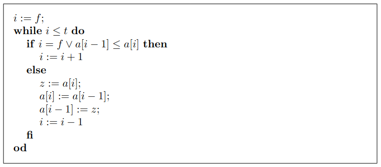
We can write down an algorithm that encodes the procedure of the gnome: see Figure 1. We are given variables \(f\) and \(t\) of type \(\mathbf{integer}\). These represent the range of indices in the array \(a\) representing the flower pots, where \(f\) is the index of the first flower pot and \(t\) is the index of the last flower pot. The variable \(i\) of type \(\mathbf{integer}\) represents the position of the gnome, and the variable \(z\) of type \(\mathbf{integer}\) is a temporary variable used for swapping the flowers.
We can make the following observations of the algorithm in Figure 1:
If \(t \leq f\) then the algorithm terminates without modifying the array. Otherwise, the bounds of the position \(i\) are: \(f\leq i\leq t+1\).
The array from \(f\) to \(i - 1\) is always sorted. This property is a loop invariant: it holds at the beginning of the loop, at the beginning of the loop body, at the end of the loop body, and after the loop.
The sorting algorithm does not insert new elements, duplicate old elements, or throw out elements: thus, the output array (that is, the value of \(a\) after running) is a permutation of the input array (the value of \(a\) before running) restricted to the given range \([f,t]\). At the beginning and end of the loop body, the current value of the array is also a restricted permutation of the input array, and this property is a loop invariant. However, this is temporarily broken when we swap around values in the array!
We now formalize the correctness proof, by means of a proof outline (see Figure 2). First, we introduce a freeze variable, the array \(b\) of type \(\mathbf{integer}\to\mathbf{integer}\). We may think of \(b\) as a snapshot of the array \(a\) at the time before running the algorithm. Since \(b\) is never modified by the program, it maintains its value over time, and thus allows us to compare the actual value of \(a\) with its original value.
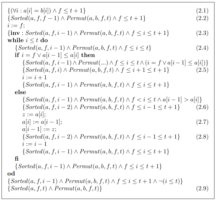
(2.1) The precondition as formulated expresses that the freeze variable \(b\) contains a snapshot of array \(a\) at this instant. Also, we restrict ourselves in this proof to the case where \(f\leq t+1\) holds (since, otherwise, the algorithm has no effect).
(2.2) This assertion follows from (2.1) since the following properties hold: \[(\forall i : a[i] = b[i]) \to \mathit{Permut}(a,b)\text{ and }\mathit{Permut}(a,b) \to \mathit{Permut}(a,b,f,t).\] We take as a witness (for the existentially quantified \(\pi\) in the definition of \(\mathit{Permut}\)) the identity function, which is a bijection. Also, the following property holds: \[t \leq f \to \mathit{Sorted}(a,f,t),\] since the range \([f,t]\) must be empty if \(t < f\), and \(\mathit{Sorted}(a,f,f)\) also holds.
(2.3) As we already observed from the algorithm, we can now formalize the loop invariant. The first part expresses that the array from \(f\) until (but excluding) \(i\) must be sorted. The second part expresses that the actual value of \(a\) is a permutation of the input array (given the name \(b\)), restricted to the range \([f,t]\). The third part expresses the bounds of the position \(i\). Note that by applying the substitution rule we obtain assertion (2.2), so we have verified that this loop invariant is initially valid. In the remainder of the proof outline we check whether the loop invariant is preserved by the loop body, and allows us to conclude our post condition.
(2.4) This assertion always holds at the start of the loop body, where we know the loop test is true. Thus we can make the invariant stronger: we know that \(i\leq t\) subsumes \(i\leq t+1\).
(2.5) We have obtained this assertion in the following way: we need to establish the loop invariant of (2.3) at the end of the loop body. Hence, it has to be a postcondition of the then-branch of the conditional statement. We apply the substitution axiom that replaces \(i\) by \(i + 1\). Now, why does this assertion follow from the preceding assertion? We discriminate two cases:
Case \(i = f\). We can establish \(\mathit{Sorted}(a,f,f)\) from the general property mentioned at (2.2).
Case \(a[i - 1] \leq a[i]\). The following property holds: \[\mathit{Sorted}(a,f,i - 1) \land a[i - 1] \leq a[i] \to \mathit{Sorted}(a,f,i)\] since we extend the range but also have the required property about \(a[i]\) and \(a[i+1]\) (and by transitivity of \(\leq\), also for all elements before \(a[i]\), cf. why the predicates \(\mathit{Sorted}\) and \(\mathit{Sorted}\,'\) are equivalent).
That \(\mathit{Permut}(a,b,f,t)\) follows from \(\mathit{Permut}(a,b,f,t)\) (shown with dots) is trivial, and it is easy to see that \(i\leq t \to i + 1 \leq t + 1\) and \(f\leq i \to f\leq i+1\).
(2.6) The assertion above this one is obtained from (2.4) and the negation of the conditional test. This assertion follows from the one above by the following argument. We have the property: \[j < i \land \mathit{Sorted}(a,f,i) \to \mathit{Sorted}(a,f,j)\] since the range becomes smaller. \(\mathit{Permut}(a,b,f,t)\) implies itself is again trivial, and \(i\leq t \to i-1 \leq t+1\) and \(f
(2.7) But how did we obtain the assertion at (2.6) in the first place? Intuitively, it is the result of swapping \(a[i]\) and \(a[i-1]\) in the assertion (2.8). Swapping does not affect \(f\leq i-1\leq t+1\). We have the following property: \[t < i \to \mathit{Sorted}(a,f,t)[a[i] := v] \equiv \mathit{Sorted}(a,f,t)\] since \(a[x][a[i] := v] = a[x]\) for all \(x < i\): there is no aliasing here!
The proof outline has a missing link: why is it that \(a\) and \(b\) are still restricted permutations when we swap \(a[i]\) and \(a[i-1]\)? The essence of the argument is that from the witness \(\pi\) of \(\mathit{Permut}(a,b,f,t)\), we can construct a new witness, say \(\pi'\), as follows: \({\pi'(i) = \pi(i - 1)}\) and \({\pi'(i-1) = \pi(i)}\) and for all other arguments \(\pi'\) and \(\pi\) agree. Further, \(i\) and \(i-1\) fall within the restricted range \([f,t]\) of the permutation.
To phrase it in a different way, we have the following property: \[\mathit{Permut}(a,b,f,t)[a[i - 1] := z][a[i] := a[i - 1]][z := a[i]] \equiv \mathit{Permut}(a,b,f,t)\] if \(f\leq i-1\leq t+1\).
(2.8) Easily obtained from the loop invariant by replacing \(i\) by \(i-1\).
(2.9) We check that the loop invariant and the negation of the loop test actually leads to the desired postcondition: we have that \(i = t + 1\) must hold.
This concludes the correctness argument of the gnome sort algorithm.
Bozosort
Bozosort is also a simple sorting algorithm. Suppose you stand in front of a table with cards on its surface, and each card has a number printed on it. Now pick any two cards on the table and swap them. Repeat this, until the numbers on the cards are all sorted from small to large. In this algorithm, we make use of a source of randomness: namely, to pick two cards to swap.
Again, we use an array \(a\) of type \(\mathbf{integer}\to\mathbf{integer}\) to represent the cards on the table. Each cell of the array corresponds to a spot on the table, and the value stored in the array is the number printed on the card.
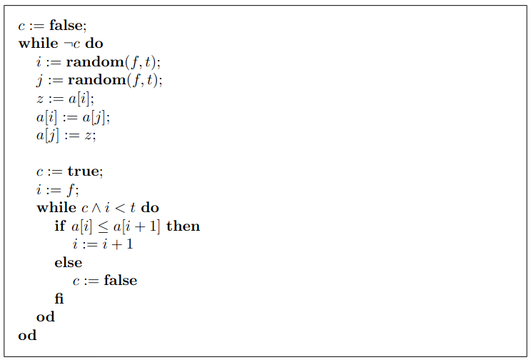
We can write down an algorithm that encodes this procedure, see Figure 3. Here, we are given variables \(f\) and \(t\) of type \(\mathbf{integer}\) representing the bounds of the array. The algorithm consists of an outer loop and an inner loop. The loop body of the outer loop has two components (separated by vertical space). By component I simply mean a subprogram. The first component chooses two random numbers and swaps the values in the array. The second component walks through the array to test whether it is actually sorted. We use the variables \(i\) and \(j\) of type \(\mathbf{integer}\), and the variable \(c\) of type \(\mathbf{boolean}\).
To understand the meaning of the random assignment, we can make use of the following axiom: \[{\{p\}\mathrel{x := {\mathbf{random}}(l,h)}\{p \land l\leq x\leq h\}}\] where \(p\) is an arbitrary formula where \(x\) does not occur free, and \(x\) does not occur in the arbitrary expressions \(l\) or \(h\). Intuitively, this statement selects (non-deterministically) an integer between \(l\) and \(h\) and updates the value of variable \(x\) with the selected value.
What happens when \(l > h\) is the case and we perform the random assignment? According to the above axiom, we obtain \[{\{l > h\}\mathrel{x := {\mathbf{random}}(l,h)}\{l > h \land l \leq x \leq h\}}.\] The postcondition is contradictory, so equivalent to \({\mathbf{false}}\). Thus, operationally, we could think that running the random assignment from such a situation is equivalent to running a program that never finishes. This works because we look at Hoare triples in their partial correctness sense.
We can make the following observations of the algorithm in Figure 3:
The actual value of array \(a\) is a permutation of the input array \(a\) at any control point, except in the middle of the first component where we perform the swapping of two elements. Thus, we could use this fact as a loop invariant of both the inner and the outer loop.
After the second component finishes its execution, the variable \(c\) represents whether the array is actually sorted or not. Hence, it is a loop invariant of the outer loop that if \(c\) is true, then the array is sorted. This means that the loop only exists when the array \(a\) is actually sorted!
The inner loop that checks whether the array is sorted looks a bit like gnome sort: the position variable \(i\) is moved to the right whenever we have tested the array elements are in order. But, instead of walking to the left, the inner loop has an early exit in case it encounters two elements that are not properly ordered. By setting \(c\) to \({\mathbf{false}}\), the outer loop must run again.
We now formalize the correctness proof, by means of a proof outline (see Figure 4). Again, we introduce a freeze variable, the array \(b\) of type \(\mathbf{integer}\to\mathbf{integer}\), with the same purpose as before.
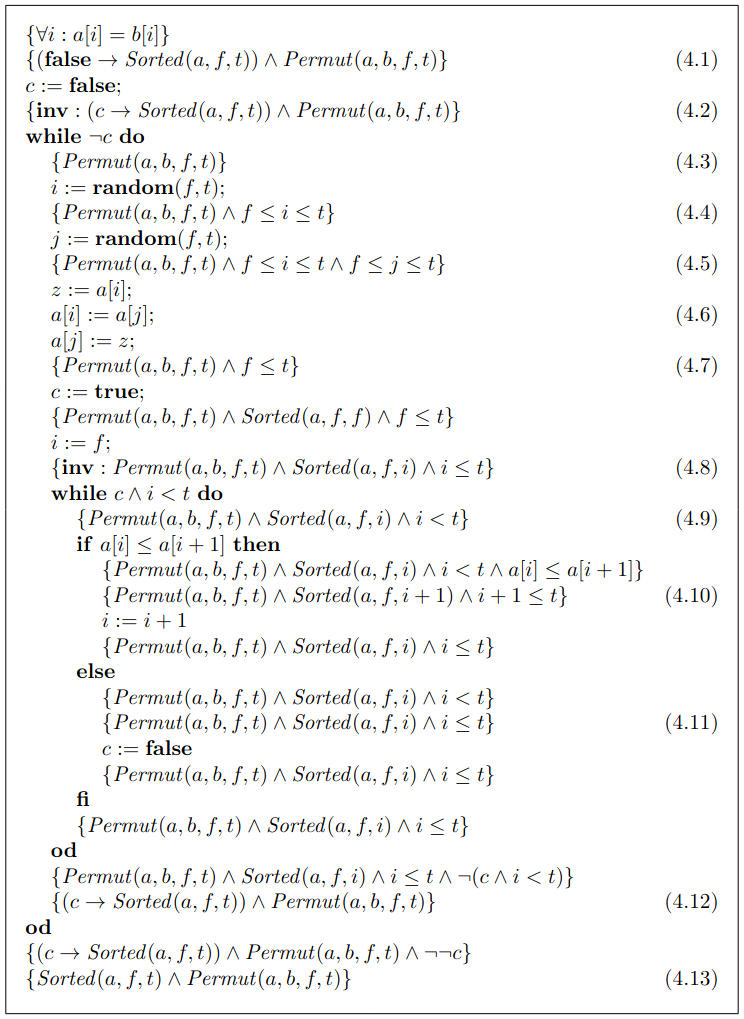
(4.1) This assertion follows from the precondition, since \(({\mathbf{false}}\to p)\) is vacuous for any formula \(p\), and the precondition implies \(\mathit{Permut}(a,b,f,t)\) for the same reason as given in (2.2).
(4.2) Here we have formalized our intuition of the loop invariant for the outer loop. Note that the assignment axiom allows us to obtain (4.1).
(4.3) When entering the loop body we know that \(c\) must be \({\mathbf{false}}\), so we can adapt the loop invariant: only information about the array \(a\) being a restricted permutation remains present here.
(4.4) Obtained by applying our axiom for random assignments.
(4.5) Also obtained by applying our axiom for random assignments. Note that from this assertion it already follows that \(f\leq t\).
(4.6) Again we have the swapping of two elements. The argument needed here is a slight generalization of the argument of (2.7) above, where the essence is this property (given \(f\leq i\leq t\) and \(f\leq j\leq t\)): \[\mathit{Permut}(a,b,f,t)[a[j] := z][a[i] := a[j]][z := a[i]] \equiv \mathit{Permut}(a,b,f,t).\] Note that if the two random variables have the same value, the swap has no effect.
(4.7) Comparing to (4.3), we now also know that \(f\leq t\). Clearly, the three preceding assignments cannot affect \(f\leq t\) and we already knew it holds in (4.5). In the other case (that \(f > t\) holds), we would not even reach this point in the program.
(4.8) We here formulate the loop invariant for the inner body. The essence is that we know that everything on the left (and including) of \(i\) must be sorted. This is initially valid, since \(\mathit{Sorted}(a,f,f)\) is true as in (2.2). We still need to establish that this is indeed a loop invariant.
(4.9) When the loop body is entered, we know both \(c\) and \(i < t\). The latter is used to make our assertion stronger than the loop invariant.
(4.10) In the case the elements are properly ordered, we can again apply the property as mentioned in the second case of (2.5).
(4.11) Easy to see that \(i
(4.12) We now establish that the outer loop invariant follows from the inner loop invariant, under the condition that the inner loop has terminated (so it’s test must be false). There are two cases:
Case \(\lnot c\): we have an early exit of the inner loop. Since \(c\) is \({\mathbf{false}}\), the left conjunct is vacuous. The right conjunct trivially follows from the inner loop invariant.
Case \(\lnot (i < t)\): we know the inner loop has fully executed, so \(i = t\) from the upper bound in the loop invariant. So \(\mathit{Sorted}(a,f,t)\) must hold, regardless of the value of \(c\).
(4.13) The postcondition is obtained by a double negation elimination on the test of the outer loop: \(\lnot\lnot c\) implies \(c\), and so from \((c\to \mathit{Sorted}(a,f,t))\) we obtain that the array is actually sorted. Again, \(\mathit{Permut}(a,b,f,t)\) follows trivially from the outer loop invariant.
This concludes the correctness argument of the bozosort algorithm.
Conclusion
We have seen two sorting algorithms, and discussed their correctness proofs. Although almost every detail is present here, there still remains a good exercise for practicing with array variable substitutions: to write down the proof outline of swapping the array elements above, and working out in all detail how it affects the restricted permutation predicate \(\mathit{Permut}\).
In this article, we only look at program correctness in the sense of partial correctness. An interesting question remains: what can we say about the termination of these algorithms? Under what conditions do these algorithms terminate? In the next following weeks of the Program Correctness course, we will look at total correctness, where we shall prove not only the correctness of a program with respect to a specification of its input and output behavior, but also whether the program terminates!
Acknowledgements. I thank Dominique Lawson and Roos Wensveen (both student assistants of the Program Correctness course) for suggesting improvements, and discovering an error in a previous version of this article. The error was that the postcondition needs to be \(\mathit{Permut}(a,b,f,t)\) and not \(\mathit{Permut}(a,b)\) (can you see why?). All remaining errors remain my own.